As the title suggests, bezier curves are AWESOME!
I was recently talking to my girlfriend, who is a super artist, and we were discussing vector images. She mentioned how difficult and EXPENSIVE it can be to create vector images, especially since you often need software like Adobe Illustrator to make high-quality SVGs.
I was intrigued by the idea that something so seemingly straightforward could be so challenging to create, so I decided to dive deeper into the mystery of vector images. It turns out that a lot of vector images are made up of n-order Bézier curves. But what exactly is a Bézier curve?
Bézier curves are essentially parametric curves defined by “control points.” The basic idea is simple: we calculate the Bézier for any given set of points, and the resulting points form the beautiful curve we see. An order-n curve will have n+1 control points. Let me illustrate with a second-order curve.
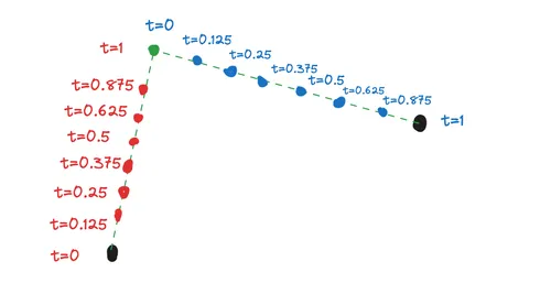
In this example, there are three points—remember, an n-order curve is defined by n+1 points. Here, the black points are the start and end points, and the green point is the control (or anchor) point. I like to think of it as a mass in space exerting some “gravitational pull” on the curve.
The Bézier function is time-dependent, or you can think of it as a step function. At each step t, we calculate:
This equation roughly translates to the distance from the start point to the end point, taken in steps of size Δt. In this case, I’ve chosen Δt as 0.125, which means we calculate the Bézier point at every 0.125 interval of t.
In the figure above, you can see a linear Bézier curve already drawn. A linear Bézier curve is simply a straight line!
Now for the fun part—how do we create a quadratic curve? We do it by recursively calculating the Bézier between each pair of Bézier points. How does this work? Check out the figure below!
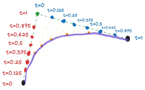
the orange points (which graph out the purple curve) are beziers taken twice. Let’s call the green anchor point P1, and the black end points as P0 and P2 respectively.
Then the bezier curve coordinates turn out to be
Pretty cool right?
Check out the demo here if you want to see bezier curves in action! eazier-bezier